title: ‘Exercise with Fractals’ teaching: 10 exercises: 50 —
- Can we tackle a real problem now?
- Create a strategy to parallelize existing code.
- Apply previous lessons.
The Mandelbrot and Julia fractals
This exercise uses Numpy and Matplotlib.
from matplotlib import pyplot as plt
import numpy as np
We will be computing the famous Mandelbrot fractal.
Complex numbers
Complex numbers are a special representation of rotations and scalings in the two-dimensional plane. Multiplying two complex numbers is the same as taking a point, rotate it by an angle \(\phi\) and scale it by the absolute value. Multiplying with a number \(z \in \mathbb{C}\) by 1 preserves \(z\). Multiplying a point at \(i = (0, 1)\) (having a positive angle of 90 degrees and absolute value 1), rotates it anti-clockwise by 90 degrees. Then you might see that \(i^2 = (-1, 0)\). The funny thing is that we can treat \(i\) as any ordinary number, and all our algebra still works out. This is actually nothing short of a miracle! We can write a complex number
\[z = x + iy,\]
remember that \(i^2 = -1\), and act as if everything is normal!
The Mandelbrot set is the set of complex numbers \[c \in \mathbb{C}\] for which the iteration
\[z_{n+1} = z_n^2 + c,\]
converges, starting from iteration at \(z_0 = 0\). We can visualize the Mandelbrot set by plotting the number of iterations needed for the absolute value \(|z_n|\) to exceed 2 (for which it can be shown that the iteration always diverges).
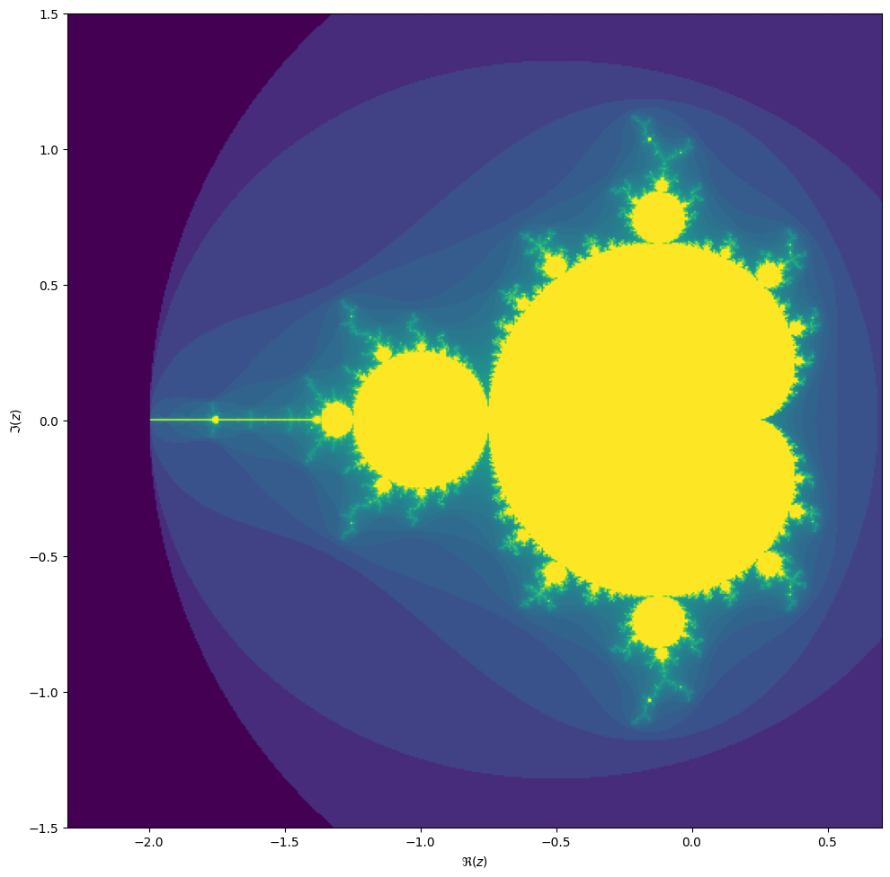
We may compute the Mandelbrot as follows:
max_iter = 256
width = 256
height = 256
center = -0.8 + 0.0j
extent = 3.0 + 3.0j
scale = max((extent / width).real, (extent / height).imag)

result = np.zeros((height, width), int)
for j in range(height):
    for i in range(width):
        c = center + (i - width // 2 + 1j * (j - height // 2)) * scale
        z = 0
        for k in range(max_iter):
            z = z**2 + c
            if (z * z.conjugate()).real > 4.0:
                break
        result[j, i] = k
Then we can plot with the following code:
fig, ax = plt.subplots(1, 1, figsize=(10, 10))
plot_extent = (width + 1j * height) * scale
z1 = center - plot_extent / 2
z2 = z1 + plot_extent
ax.imshow(result**(1 / 3), origin='lower', extent=(z1.real, z2.real, z1.imag, z2.imag))
ax.set_xlabel("$\Re(c)$")
ax.set_ylabel("$\Im(c)$")
Things become really loads of fun when we zoom in. We can play around
with the center and extent values, and
necessarily max_iter, to control our window:
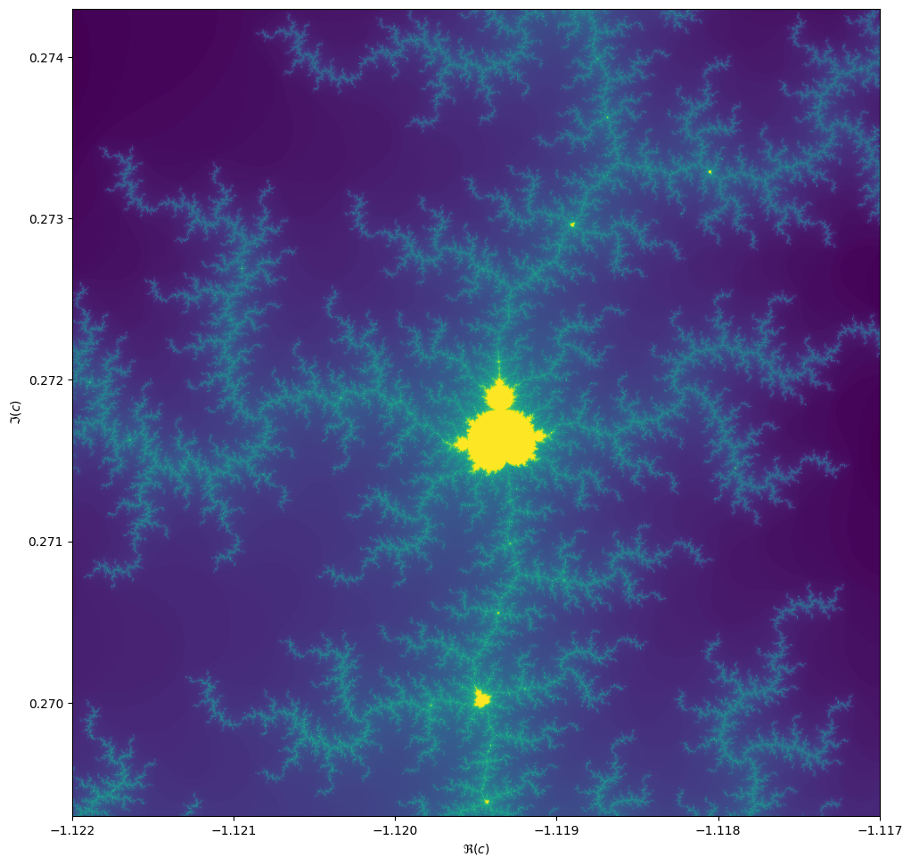
max_iter = 1024
center = -1.1195 + 0.2718j
extent = 0.005 + 0.005j
When we zoom in on the Mandelbrot fractal, we get smaller copies of the larger set!
Exercise
Turn this into an efficient parallel program. What kind of speed-ups do you get?
Solution
Create a BoundingBox class
We start with a naive implementation. It may be convenient to define
a BoundingBox class in a separate module
bounding_box.py. We add methods to this class later on.
from dataclasses import dataclass
from typing import Optional
import numpy as np
import dask.array as da


@dataclass
class BoundingBox:
    width: int
    height: int
    center: complex
    extent: complex
    _scale: Optional[float] = None

    @property
    def scale(self):
        if self._scale is None:
            self._scale = max(self.extent.real / self.width,
                              self.extent.imag / self.height)
        return self._scale

    <<bounding-box-methods>>

test_case = BoundingBox(1024, 1024, -1.1195+0.2718j, 0.005+0.005j)
Solution
Plotting function
import matplotlib  # type:ignore
matplotlib.use(backend="Agg")
from matplotlib import pyplot as plt
import numpy as np

from bounding_box import BoundingBox

def plot_fractal(box: BoundingBox, values: np.ndarray, ax=None):
    if ax is None:
        fig, ax = plt.subplots(1, 1, figsize=(10, 10))
    else:
        fig = None
    plot_extent = (box.width + 1j * box.height) * box.scale
    z1 = box.center - plot_extent / 2
    z2 = z1 + plot_extent
    ax.imshow(values, origin='lower', extent=(z1.real, z2.real, z1.imag, z2.imag),
              cmap=matplotlib.colormaps["viridis"])
    ax.set_xlabel("$\Re(c)$")
    ax.set_ylabel("$\Im(c)$")
    return fig, ax
Solution
Some solutions
The natural approach with Python is to speed this up with Numba.
Then, there are three ways to parallelize: first, letting Numba
parallelize the function; second, doing a manual domain decomposition
and using one of the many Python ways to run multi-threaded things;
third, creating a vectorized function and parallelizing it using
dask.array. This last option is almost always slower than
@njit(parallel=True) and domain decomposition.
Solution
Numba (serial)
When we port the core Mandelbrot function to Numba, we need to keep some best practices in mind:
- Don’t pass composite objects other than Numpy arrays.
- Avoid acquiring memory inside a Numba function; rather, create an array in Python and then pass it to the Numba function.
- Write a Pythonic wrapper around the Numba function for easy use.
from typing import Any, Optional
import numba  # type:ignore
import numpy as np

from bounding_box import BoundingBox


@numba.njit(nogil=True)
def compute_mandelbrot_numba(
        result, width: int, height: int, center: complex,
        scale: complex, max_iter: int):
    for j in range(height):
        for i in range(width):
            c = center + (i - width // 2 + 1j * (j - height // 2)) * scale
            z = 0.0 + 0.0j
            for k in range(max_iter):
                z = z**2 + c
                if (z * z.conjugate()).real >= 4.0:
                    break
            result[j, i] = k
    return result


def compute_mandelbrot(
        box: BoundingBox, max_iter: int,
        result: Optional[np.ndarray[np.int64]] = None,
        throttle: Any = None):
    result = result if result is not None \
            else np.zeros((box.height, box.width), np.int64)
    return compute_mandelbrot_numba(
        result, box.width, box.height, box.center, box.scale,
        max_iter=max_iter)
Numba parallel=True
We can parallelize loops directly with Numba. Pass the flag
parallel=True and use prange to create the
loop. Here, it is even more important to obtain the result array outside
the context of Numba, otherwise the result will be slower than the
serial version.
from typing import Optional
import numba  # type:ignore
from numba import prange  # type:ignore
import numpy as np

from .bounding_box import BoundingBox


@numba.njit(nogil=True, parallel=True)
def compute_mandelbrot_numba(
        result, width: int, height: int, center: complex, scale: complex,
        max_iter: int):
    for j in prange(height):
        for i in prange(width):
            c = center + (i - width // 2 + (j - height // 2) * 1j) * scale
            z = 0.0+0.0j
            for k in range(max_iter):
                z = z**2 + c
                if (z*z.conjugate()).real >= 4.0:
                    break
            result[j, i] = k
    return result


def compute_mandelbrot(box: BoundingBox, max_iter: int,
                       throttle: Optional[int] = None):
    if throttle is not None:
        numba.set_num_threads(throttle)
    result = np.zeros((box.height, box.width), np.int64)
    return compute_mandelbrot_numba(
        result, box.width, box.height, box.center, box.scale,
        max_iter=max_iter)
Solution
Domain splitting
We split the computation into a set of sub-domains. The
BoundingBox.split() method is designed so that, if we
deep-map the resulting list-of-lists, we can recombine the results using
numpy.block().
def split(self, n):
    """Split the domain in nxn subdomains, and return a grid of BoundingBoxes."""
    w = self.width // n
    h = self.height // n
    e = self.scale * w + self.scale * h * 1j
    x0 = self.center - e * (n / 2 - 0.5)
    return [[BoundingBox(w, h, x0 + i * e.real + j * e.imag * 1j, e)
             for i in range(n)]
            for j in range(n)]
To perform the computation in parallel, let’s go ahead and choose the
most difficult path: asyncio. There are other ways to do
this, like setting up a number of threads or using Dask. However,
asyncio is available in Python natively. In the end, the
result is very similar to what we would get using
dask.delayed.
This may seem as a lot of code, but remember: we only use Numba to compile the core part and then Asyncio to parallelize. The progress bar is a bit of flutter and the semaphore is only there to throttle the computation to fewer cores. Even then, this solution is the most extensive by far but also the fastest.
from typing import Optional
import numpy as np
import asyncio
from psutil import cpu_count  # type:ignore
from contextlib import nullcontext

from .bounding_box import BoundingBox
from .numba_serial import compute_mandelbrot as mandelbrot_serial


async def a_compute_mandelbrot(
        box: BoundingBox,
        max_iter: int,
        semaphore: Optional[asyncio.Semaphore]):
    async with semaphore or nullcontext():
        result = np.zeros((box.height, box.width), np.int64)
        await asyncio.to_thread(
                mandelbrot_serial, box, max_iter, result=result)
    return result


async def a_domain_split(box: BoundingBox, max_iter: int,
                         sem: Optional[asyncio.Semaphore]):
    n_cpus = cpu_count(logical=True)
    split = box.split(n_cpus)
    split_result = await asyncio.gather(
        *(asyncio.gather(
            *(a_compute_mandelbrot(b, max_iter, sem)
              for b in row))
          for row in split))
    return np.block(split_result)


def compute_mandelbrot(box: BoundingBox, max_iter: int,
                       throttle: Optional[int] = None):
    sem = asyncio.Semaphore(throttle) if throttle is not None else None
    return asyncio.run(a_domain_split(box, max_iter, sem))
Solution
Numba vectorize
Another solution is to use Numba’s @guvectorize
decorator. The speed-up (on my machine) is not as dramatic as with the
domain decomposition, though.
def grid(self):
    """Return the complex values on the grid in a 2d array."""
    x0 = self.center - self.extent / 2
    x1 = self.center + self.extent / 2
    g = np.mgrid[x0.imag:x1.imag:self.height*1j,
                 x0.real:x1.real:self.width*1j]
    return g[1] + g[0]*1j

def da_grid(self):
    """Return the complex values on the grid in a 2d array."""
    x0 = self.center - self.extent / 2
    x1 = self.center + self.extent / 2
    x = np.linspace(x0.real, x1.real, self.width, endpoint=False)
    y = np.linspace(x0.imag, x1.imag, self.height, endpoint=False)
    g = da.meshgrid(x, y)
return g[1] + g[0]*1jfrom typing import Any
from numba import guvectorize, int64, complex128 # type:ignore
import numpy as np
from .bounding_box import BoundingBox
@guvectorize([(complex128[:, :], int64, int64[:, :])],
"(n,m),()->(n,m)",
nopython=True)
def compute_mandelbrot_numba(inp, max_iter: int, result):
for j in range(inp.shape[0]):
for i in range(inp.shape[1]):
c = inp[j, i]
z = 0.0+0.0j
for k in range(max_iter):
z = z**2 + c
if (z*z.conjugate()).real >= 4.0:
break
result[j, i] = k
def compute_mandelbrot(box: BoundingBox, max_iter: int, throttle: Any = None):
result = np.zeros((box.height, box.width), np.int64)
c = box.grid()
compute_mandelbrot_numba(c, max_iter, result)
return resultSolution
Benchmarks

from typing import Optional
import timeit
from . import numba_serial, numba_parallel, vectorized, domain_splitting
from .bounding_box import BoundingBox, test_case


compile_box = BoundingBox(16, 16, 0.0+0.0j, 1.0+1.0j)
timing_box = test_case


def compile_run(m):
    m.compute_mandelbrot(compile_box, 1)


def timing_run(m, throttle: Optional[int] = None):
    m.compute_mandelbrot(timing_box, 1024, throttle=throttle)


modules = ["numba_serial:1", "vectorized:1"] \
        + [f"domain_splitting:{n}" for n in range(1, 9)] \
        + [f"numba_parallel:{n}" for n in range(1, 9)]


if __name__ == "__main__":
    with open("timings.txt", "w") as out:
        headings = ["name", "n", "min", "mean", "max"]
        print(f"{headings[0]:<20}" \
              f"{headings[1]:>10}" \
              f"{headings[2]:>10}" \
              f"{headings[3]:>10}" \
              f"{headings[4]:>10}",
              file=out)
        for mn in modules:
            m, n = mn.split(":")
            n_cpus = int(n)
            setup = f"from mandelbrot.bench_all import timing_run, compile_run\n" \
                    f"from mandelbrot import {m}\n" \
                    f"compile_run({m})"
            times = timeit.repeat(
                stmt=f"timing_run({m}, {n_cpus})",
                setup=setup,
                number=1,
                repeat=50)
            print(f"{m:20}" \
                  f"{n_cpus:>10}" \
                  f"{min(times):10.5g}" \
                  f"{sum(times)/len(times):10.5g}" \
                  f"{max(times):10.5g}",
                  file=out)

    import pandas as pd
    from plotnine import ggplot, geom_point, geom_ribbon, geom_line, aes
    timings = pd.read_table("timings.txt", delimiter=" +", engine="python")
    plot = ggplot(timings, aes(x="n", y="mean", ymin="min", ymax="max",
                               color="name", fill="name")) \
        + geom_ribbon(alpha=0.3, color="none") \
        + geom_point() + geom_line()
    plot.save("mandelbrot-timings.svg")
Extra: Julia sets
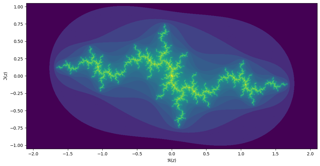
For each value \[c\] we can compute the Julia set, namely the set of starting values \[z_1\] for which the iteration over \[z_{n+1}=z_n^2 + c\] converges. Every location on the Mandelbrot image corresponds to its own unique Julia set.
max_iter = 256
center = 0.0+0.0j
extent = 4.0+3.0j
scale = max((extent / width).real, (extent / height).imag)

result = np.zeros((height, width), int)
c = -1.1193+0.2718j

for j in range(height):
    for i in range(width):
        z = center + (i - width // 2 + (j - height // 2)*1j) * scale
        for k in range(max_iter):
            z = z**2 + c
            if (z * z.conjugate()).real > 4.0:
                break
        result[j, i] = k
If we take the centre of the last image, we get the following rendering of the Julia set:
Generalize
Can you generalize your Mandelbrot code to compute both the Mandelbrot and the Julia sets efficiently, while reusing as much code as possible?
- Actually making code faster is not always straightforward.
- Easy one-liners can get you 80% of the way.
- Writing clean and modular code often makes parallelization easier later on.