How do we know whether our program ran faster in parallel?
How do we appraise efficiency?

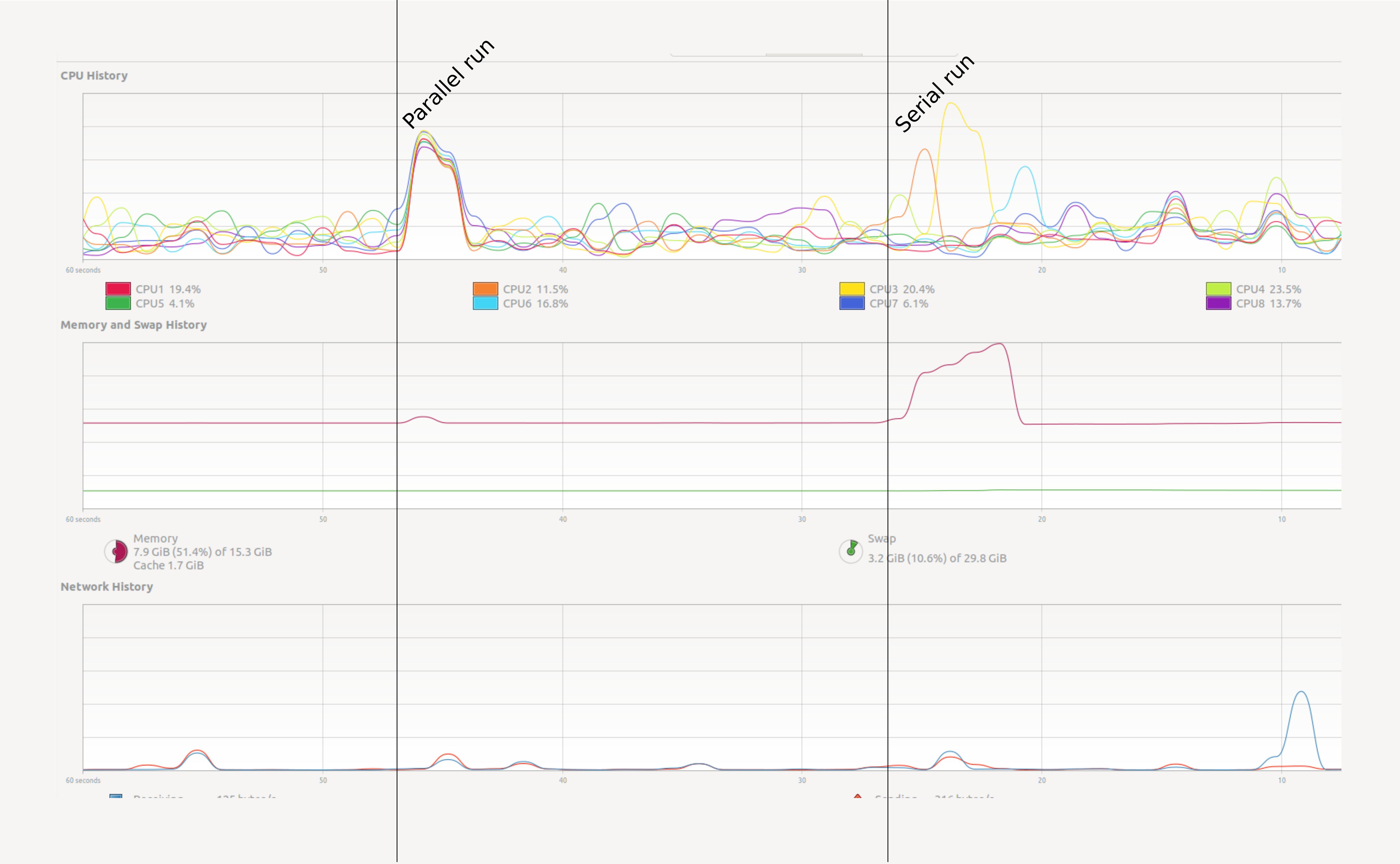
View performance on system monitor.
Find out how many cores your machine has.
Use %time and %timeit line-magic.
Use a memory profiler.
Plot performance against number of work units.
Understand the influence of hyper-threading on timings.

A first example with Dask

We will create parallel programs in Python later. First let’s see a small example. Open your System Monitor (the application will vary between specific operating systems), and run the following code examples:

# Summation making use of numpy:
import numpy as np
result = np.arange(10**7).sum()

# The same summation, but using dask to parallelize the code.
# NB: the API for dask arrays mimics that of numpy
import dask.array as da
work = da.arange(10**7).sum()
result = work.compute()

Try a heavy enough task

Your system monitor may not detect so small a task. In your computer you may have to gradually raise the problem size to 10**8 or 10**9 to observe the effect in long enough a run. But be careful and increase slowly! Asking for too much memory can make your computer slow to a crawl.

screenshot of system monitor — System monitor

How can we monitor this more conveniently? In Jupyter we can use some line magics, small “magic words” preceded by the symbol %% that modify the behaviour of the cell.

%%time
np.arange(10**7).sum()

The %%time line magic checks how long it took for a computation to finish. It does not affect how the computation is performed. In this regard it is very similar to the time shell command.

If we run the chunk several times, we will notice variability in the reported times. How can we trust this timer, then? A possible solution will be to time the chunk several times, and take the average time as our valid measure. The %%timeit line magic does exactly this in a concise and convenient manner! %%timeit first measures how long it takes to run a command once, then repeats it enough times to get an average run-time. Also, %%timeit can measure run times discounting the overhead of setting up a problem and measuring only the performance of the code in the cell. So this outcome is more trustworthy.

%%timeit
np.arange(10**7).sum()

You can store the output of %%timeit in a Python variable using the -o flag:

time = %timeit -o np.arange(10**7).sum()
print(f"Time taken: {time.average:.4f} s")

Note that this metric does not tell you anything about memory consumption or efficiency.

Timeit

Use timeit to time the following snippets:

[x**2 for x in range(100)]

map(lambda x: x**2, range(100))

Can you explain the difference? How about the following

for x in range(100):
    x**2

Is that faster than the first one? Why?

Solution

Python’s map function is lazy. It won’t compute anything until you iterate it. Try list(map(...)). The third example doesn’t allocate any memory, which makes it faster.

Memory profiling

Benchmarking is the action of systematically testing performance under different conditions.
Profiling is the analysis of which parts of a program contribute to the total performance, and the identification of possible bottlenecks.

We will use the package memory_profiler to track memory usage. It can be installed executing the code below in the console:

pip install memory_profiler

The memory usage of the serial and parallel versions of a code will vary. In Jupyter, type the following lines to see the effect in the code presented above (again, increase the baseline value 10**7 if needed):

import numpy as np
import dask.array as da
from memory_profiler import memory_usage
import matplotlib.pyplot as plt

def sum_with_numpy():
    # Serial implementation
    np.arange(10**7).sum()

def sum_with_dask():
    # Parallel implementation
    work = da.arange(10**7).sum()
    work.compute()

memory_numpy = memory_usage(sum_with_numpy, interval=0.01)
memory_dask = memory_usage(sum_with_dask, interval=0.01)

# Plot results
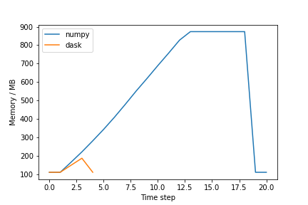
plt.plot(memory_numpy, label='numpy')
plt.plot(memory_dask, label='dask')
plt.xlabel('Interval counter [-]')
plt.ylabel('Memory usage [MiB]')
plt.legend()
plt.show()

The plot should be similar to the one below:

showing very high peak for numpy, and constant low line for dask — Memory performance

Exercise (plenary)

Why is the Dask solution more memory-efficient?

Solution

Chunking! Dask chunks the large array so that the data is never entirely in memory.

Profiling from Dask

Dask has several built-in option for profiling. See the dask documentation for more information.

Using many cores

Using more cores for a computation can decrease the run time. The first question is of course: how many cores do I have? See the snippet below to find this out:

Find out the number of cores in your machine

The number of cores can be found from Python upon executing:

import psutil
N_physical_cores = psutil.cpu_count(logical=False)
N_logical_cores = psutil.cpu_count(logical=True)
print(f"The number of physical/logical cores is {N_physical_cores}/{N_logical_cores}")

Usually the number of logical cores is higher than the number of physical cores. This is due to hyper-threading, which enables each physical CPU core to execute several threads at the same time. Even with simple examples, performance may scale unexpectedly. There are many reasons for this, hyper-threading being one of them. See the ensuing example.

On a machine with 4 physical and 8 logical cores, this admittedly over-simplistic benchmark:

x = []
for n in range(1, 9):
    time_taken = %timeit -r 1 -o da.arange(5*10**7).sum().compute(num_workers=n)
    x.append(time_taken.average)

gives the result:

import pandas as pd
data = pd.DataFrame({"n": range(1, 9), "t": x})
data.set_index("n").plot()

showing that using more cores can also make things slower — Timings against number of cores

Discussion

Why does the runtime increase if we add more than 4 cores? This has to do with hyper-threading. On most architectures it does not make much sense to use more workers than the physical cores you have.

Profiling

Types

There are two types of profiling approaches - deterministic and statistical. The deterministic profiling works by hooking into function calls, function returns, and/or leave events and collecting relevant metrics, e.g. precise timing, for the intervals between these events. In contrast, the statistical profiling randomly samples metrics during the execution of the user’s code. Due to its nature, the statistical profiling provides only relative information about the consumed resources.

In general, the statistical technique imposes less overhead and, therefore, is considered to be more suitable for “heavy” codes. It also comes in handy when getting a first “high-level” overview of the profiled application. It is worth noting, however, that some profilers allow adjustment of the sampling rate, which may lead to an increase in the added overhead.

Basics time measurement

The most basic deterministic way of profiling an application is by measuring its execution time or elapsed time of an individual function. Usually one would like to start with high-level functions, narrowing down the evaluation scope to detect the most time-consuming piece of the code.

The time Python module provides a straightforward way to measure elapsed time:

import time

def some_function():
    # Example function to measure
    total = 0
    for i in range(1, 1000000):
        total += i
    return total

# Measure elapsed time
start_time = time.time()  # Record start time
result = some_function()  # Call the function
end_time = time.time()    # Record end time

elapsed_time = end_time - start_time  # Calculate elapsed time
print(f"Elapsed time: {elapsed_time:.4f} seconds")

An example output:

Elapsed time: 0.0586 seconds

Here, we measure the elapsed time of the some_function function by recording times before the function call and after the function call using the Python time() function. This function returns the number of seconds passed since the epoch. To calculate the elapsed time we simply subtract the start_time from the end_time.

Alternatively, one can use the timeit Python module:

import timeit

def some_function():
    total = 0
    for i in range(1, 1000000):
        total += i
    return total

# Measure elapsed time
elapsed_time = timeit.timeit(some_function, number=1)  # Run function once
print(f"Elapsed time: {elapsed_time:.4f} seconds")

The timeit module is designed for more accurate timing, especially for short code snippets. This is achieved by: - repeating tests multiple times in order to eliminate interference from other processes (e.g. OS processes) - disabling the garbage collector to eliminate possible execution of this mechanism during the time measurement step - relying on the most accurate timer available at the OS level.

Using the code snippets from above, try incorporating both methods into one script and see which one reports a smaller elapsed time.

Profiling tools

There is a great variety of profiling tools available for Python applications. Generally, they differ by the type of profiling technique used - deterministic or statistical, and by the type of data analyzed - time, memory or network communication. Below is a short list of the most common profiling tools:

Type	Tool	Purpose
Standard Profilers	`cProfile`	A built-in Python module for profiling function calls and execution time.
	`profile`	Similar to cProfile, but written in pure Python (slower, more flexible).
Memory Profilers	`memory_profiler`	Monitors memory usage of Python code, line-by-line.
	`objgraph`	Visualizes Python object graphs to track references and memory leaks.
	`tracemalloc`	Built-in module to track memory allocations.
Line Profilers	`line_profiler`	Profiles time spent on each line of code.
	`Py-Spy`	Low-overhead sampling profiler for live Python processes, with flamegraph support.
Parallel and Multithreading Profilers	`pyinstrument`	Records and visualizes profiling sessions, optimized for async and multi-threaded code.
	`scalene`	Profiles Python programs focusing on CPU, memory, and GPU usage, with multithreading support.
	`yappi`	High-performance multi-threaded profiler.

Some of these profilers (pyinstrument, yappi, memory_profiler, line-profiler) are available on Snellius under the decoProf/0.0.1-GCCcore-12.3.0 module in the 2023 environment:

$ module purge
$ module load 2023
$ module load decoProf/0.0.1-GCCcore-12.3.0

In this tutorial we will cover only some of them.

cProfile

The most standard profiling tool for Python is cProfile. This deterministic tool is used for detailed profiling of a function or program, breaking down where the time is spent. The usage is as follows:

import time
import cProfile

def some_function():
    # Example function to measure
    total = 0
    for i in range(1, 1000000):
        total += i
    return total

# Profile `some_function`
cProfile.run('some_function()')

An example output:

         4 function calls in 0.078 seconds

   Ordered by: standard name

   ncalls  tottime  percall  cumtime  percall filename:lineno(function)
        1    0.000    0.000    0.078    0.078 <string>:1(<module>)
        1    0.078    0.078    0.078    0.078 time.py:5(some_function)
        1    0.000    0.000    0.078    0.078 {built-in method builtins.exec}
        1    0.000    0.000    0.000    0.000 {method 'disable' of '_lsprof.Profiler' objects}

As you can see, cProfile reports more metrics, compared to time or timeit modules. However, the reported times are also higher, indicating a significant overhead imposed by the profiler.

Among the reported values one can see: - the number of calls for a function (ncalls) - the total time spent a function (tottime) and the corresponding average time per call (percall) - cumulative time spent by a function, i.e. the total time spent in a function plus all functions that that function called (cumtime) and the corresponding average time per call (percall) - file name and the line number per function

Analyzing the example output from above we can see that the most time (0.078 seconds) was spent in some_function located on line 5 in file time.py.

Using the code snippet from this section, implement a nested function with heavy workload in some_function and profile the application. Take a look at the generated report and and analise it.

memory_profiler

The memory_profiler allows monitoring of the memory footprint of a Python application. It helps to detect memory-intensive operations and identify memory leaks or unnecessary memory retention. To use it one needs to add a decorator @profile in front of the function declaration in the source code. For instance:

from memory_profiler import profile

@profile
def some_function():
    # Allocate some memory
    large_list = [i ** 2 for i in range(10**5)]   # Creates a large list
    del large_list                                # Deletes the list
    another_list = [j / 2 for j in range(10**5)]  # Creates another list
    return another_list

if __name__ == "__main__":
    some_function()

To run memory_profiler one can use the command-line tool mprof:

$ mprof run mem.py

This command will generate and print a detailed report of the line-by-line memory usage in a function of interest, e.g.:

Line #    Mem usage    Increment  Occurrences   Line Contents
=============================================================
     3     23.3 MiB     23.3 MiB           1   @profile
     4                                         def some_function():
     5                                             # Allocate some memory
     6     27.3 MiB      4.0 MiB      100003       large_list = [i ** 2 for i in range(10**5)]  # Creates a large list
     7     25.4 MiB     -1.9 MiB           1       del large_list                              # Deletes the list
     8     26.4 MiB      1.0 MiB      100003       another_list = [j / 2 for j in range(10**5)]  # Creates another list
     9     26.4 MiB      0.0 MiB           1       return another_list

After the report is generated, it’s also possible generate a memory footprint over time plot using the mprof plot command:

$ mprof plot -o img.jpeg

Alternatively, one can also ask Python to execute a script using the memory_profiler module:

$ python -m memory_profiler mem.py

Using the code snippet from this section, perform memory profiling of the code and visualize the memory footprint using the mprof plot command.

line_profiler

The line_profiler tool helps to pinpoint specific lines of code that are bottlenecks and useful for functions or loops with high computational overhead. It will profile the time individual lines of code take to execute. To enable the profiler on a function, one can use the @profile decorator.

As an example, we will use similar script as we used in the cProfile section:

@profile
def some_function():
    # Example function to measure
    total = 0
    for i in range(1, 1000000):
        total += i
    return total

some_function()

To execute the line_profiler we use the kernprof command, which is part of the line_profiler package:

$ kernprof -l -v time.py

where the -l option enables line-by-line profiling, and the -v option displays the profiling results after execution.

An example output:

Wrote profile results to time.py.lprof
Timer unit: 1e-06 s

Total time: 0.426888 s
File: time.py
Function: some_function at line 5

Line #      Hits         Time  Per Hit   % Time  Line Contents
==============================================================
     5                                           @profile
     6                                           def some_function():
     7                                               # Example function to measure
     8         1          2.1      2.1      0.0      total = 0
     9   1000000     192291.7      0.2     45.0      for i in range(1, 1000000):
    10    999999     234593.6      0.2     55.0          total += i
    11         1          0.2      0.2      0.0      return total

Here Hits represents the number of times the line was executed, Time shows the total time spent on that line (in microseconds), Per Hit shows an average time per execution of the line, % Time indicates percentage of total time spent on the line, Line Contents shows the actual line of code being profiled.

yappi

yappi is a deterministic profiling tool that allows the profiling of multi-threaded applications. Unlike previous tools, it doesn’t use decorators. Instead, it requires wrapping a call for a function of interest with yappi profiling functions. For instance:

import yappi

def some_function():
    # Example function to measure
    total = 0
    for i in range(1, 1000000):
        total += i
    return total

# Start yappi profiling
yappi.start()

# Run the function
some_function()

# Stop profiling
yappi.stop()

# Print function-level statistics
yappi.get_func_stats().print_all()

# Optional: Print thread-level stats if applicable
yappi.get_thread_stats().print_all()

To run profiling and get metrics we only need to execute our script as usual:

$ python time.py

An example output:

Clock type: CPU
Ordered by: totaltime, desc

name                                  ncall  tsub      ttot      tavg
..tmp/python/time.py:6 some_function  1      0.079182  0.079182  0.079182

name           id     tid              ttot      scnt
_MainThread    0      23313336990592   0.079193  1

Here, ncall shows the number of times the function was called, tsub shows time spent in the function itself (excluding calls to other functions), ttot indicates the total time spent in the function (including calls to other functions), and tavg shows the average time per function call. At the end of the report we can see information about the spawned threads: tid indicates the thread ID, ttot shows how much time this thread has spent in total, and scnt shows how many times this thread was scheduled.

Let’s use the previous example and spawn a few threads to see how yappi’s output will change:

import yappi
import threading

num_threads = 2

def some_function():
    # Example function to measure
    total = 0
    for i in range(1, 1000000):
        total += i
    return total

# Start yappi profiling
yappi.start()

threads_lst = []

# generate threads
for i in range(num_threads):
    thr = threading.Thread(target=some_function)
    thr.start()
    threads_lst.append(thr)
# wait all threads to finish
for thr in threads_lst:
    thr.join()

# Stop profiling
yappi.stop()

# Print function-level statistics
yappi.get_func_stats().print_all()

# Optional: Print thread-level stats if applicable
yappi.get_thread_stats().print_all()

Here we define the number of threads with the num_threads variable. Instead of calling for some_function we now spawn num_threads threads and ask each thread to run it. We call for the join() method to ensure that all threads have finished their work.

An example output:

Clock type: CPU
Ordered by: totaltime, desc

name                                  ncall  tsub      ttot      tavg
..ib/python3.11/threading.py:964 run  2      0.000019  0.158632  0.079316
../python/threads.py:6 some_function  2      0.158613  0.158613  0.079306
..3.11/threading.py:938 Thread.start  2      0.000022  0.000289  0.000144
..3.11/threading.py:1080 Thread.join  2      0.000021  0.000189  0.000094
..:1118 Thread._wait_for_tstate_lock  2      0.000031  0.000159  0.000079
..on3.11/threading.py:604 Event.wait  2      0.000020  0.000120  0.000060
..1/threading.py:849 Thread.__init__  2      0.000035  0.000091  0.000046
..11/threading.py:288 Condition.wait  2      0.000028  0.000086  0.000043
...11/threading.py:1044 Thread._stop  2      0.000035  0.000074  0.000037
..ng.py:822 _maintain_shutdown_locks  2      0.000013  0.000032  0.000016
..1/threading.py:1071 Thread._delete  2      0.000028  0.000031  0.000016
..11/threading.py:555 Event.__init__  2      0.000011  0.000024  0.000012
..1/threading.py:1446 current_thread  4      0.000011  0.000015  0.000004
..on3.11/threading.py:832 <listcomp>  2      0.000010  0.000014  0.000007
..3.11/_weakrefset.py:85 WeakSet.add  2      0.000011  0.000012  0.000006
..hreading.py:236 Condition.__init__  2      0.000011  0.000011  0.000006
..ing.py:273 Condition._release_save  2      0.000005  0.000007  0.000003
..hreading.py:267 Condition.__exit__  2      0.000005  0.000007  0.000003
..reading.py:264 Condition.__enter__  2      0.000005  0.000006  0.000003
..reading.py:279 Condition._is_owned  2      0.000004  0.000006  0.000003
..thon3.11/threading.py:804 _newname  2      0.000006  0.000006  0.000003
...py:276 Condition._acquire_restore  2      0.000004  0.000006  0.000003
..reading.py:1199 _MainThread.daemon  4      0.000005  0.000005  0.000001
..ng.py:1317 _make_invoke_excepthook  2      0.000004  0.000004  0.000002
..3.11/threading.py:568 Event.is_set  4      0.000003  0.000003  0.000001

name           id     tid              ttot      scnt
Thread         2      22506480539200   0.079892  2
Thread         1      22506482656832   0.078816  2
_MainThread    0      22506711391104   0.000629  5

The report now lists multiple calls for the threading module which makes analysis a bit harder. However, both tables are sorted by the ttot column, which helps us to identify that most of the time was spent in the some_function function. Also, the second table shows that each thread took an equal amount of work, which is generally good for multithreaded applications.

Using the code snippet with threads from this section, increase the number of threads and perfom profiling of the code.

Understanding performance is often non-trivial.
Memory is just as important as speed.
To measure is to know.